Time Series Regression Models

Joe Lee,Tue Aug 06 2024•time_series

Linear Regression models

\begin{matrix} (7.1) & y_{t} = β_{0} + β_{1} x_{1, t} + β_{2} x_{2, t} + \dots + β_{k} x_{k, t} + ε_{t}, \end{matrix}

Linear regression models estimates the coefficient of the explanatory variables (x) in order to minimize the SSE, which is also known as the Least Squares Estimation.
In R, the code can be written as below, which provides the estimated coefficients.

Data |> model(TSML(Value ~ x1 + x2 + ...))

A good method to evaluate the model is to check the goodness of fit, also known as R^2 or adjusted R^2, which takes in to account of the number of explanatory variables.
R^2 measures the proportion of variance in the forecasts over the total variance; in simpler terms, the amount of variability the forecasts explain from the regression model from the actual data.

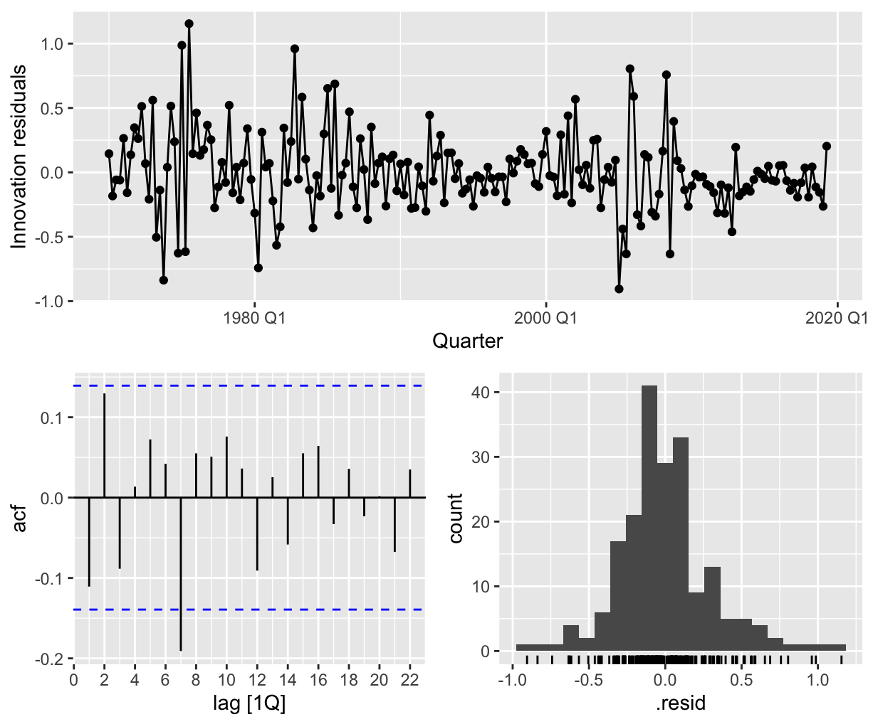
The key assumptions for a regression model is that the residuals are normally distributed and that the explanatory variables are not correlated; thus it is important to verify that these assumptions holds.
An easy way to generate the graphs for residual analysis is gg_tsresiduals().

We should check that the residuals are normally distributed through the histogram, and that the residuals do not display any seasonal component in the ACF plot.
Addition to the ACF plot, the Ljung-Box test checks whether the residuals displays no autocorrelation for lags by the code below.

Data |> features(.innov, ljung_box, lag = 5)

To check whether the residuals are randomly distributed, we can plot scatterplots of residuals v.s explanatory variables and residuals v.s variables not in model to check whether there are some patterns in the residuals.
To check whether residuals have constant variance, we can plot the residuals against the fitted values.

Dummy variables can be utilized to represent certain explanatory variables.
For example, dummy variables for each Year, Quarter, Month, or week can represent the effect for that specific time.
Dummy variables can also represent an outlier, such as a holiday or leap years.
Instead of utilizing dummy variables for seasonality, harmonic regression can be used to approximate seasonal periods.
Harmonic regression utilizes a Fourier Series, which can approximate any period function bny adjusting its K value. As they require fewer variables, they can be helpful for seasonalities that require many dummy variables.
As the value of K increases, the Fourier Series captures more complexity of the data.

$SSE = \sum_{t = 1}^{T} e_{t}^{2} .$
As discussed earlier the measure of fit is one of the ways to validate a good model, which is equivalent to minimizing the SSE.
An adjusted R^2 takes into account the number of explanatory variables-less variables have a higher R^2 value. This overcomes the property of R^2 increasing with the addition of any explanatory variables, even if the variable itself is insignificant.

Cross validation comes from making one-step or multi-step forecasts into the future sets within the sample and calculating the MSE from the errors during the process.
It is also possible to utilize a leave-on-out cross-validation for faster calculations.

$AIC = T \log (\frac{SSE}{T}) + 2 (k + 2),$
Where T is the number of observations in the estimations and k is the number of explanatory variables.
AIC penalizes the fit of the model (SSE) to the number of parameters that needed to be estimated.
AICc is used for smaller values of T as AIC selects too many predictors.
AIC is asymptotically equivalent to minimizing the MSE.
It is also similiar to leave-one-out cross-validation.

$BIC = T \log (\frac{SSE}{T}) + (k + 2) \log (T) .$
The BIC utilizes the same concept as the AIC but penalizes any extra explanatory variables than the AIC.
The BIC is similar to leave-v-out cross-validation.

It is important to note that selecting predictors based on these methods invalidates any assumptions for any statistical testing that is to be conducted on the model.