Exponential Smoothing / ETS model forecasting

Simple Exponential Smoothing :

• $\begin{array}{}\text{(8.1)}& {\hat{y}}_{T+1|T}=\alpha y_T+\alpha (1-\alpha )y_{T-1}+\alpha (1-\alpha {)}^2{y}_{T-2}+\cdots ,\end{array}$

• Simple exponential smoothing models take account of historial data and apply a moving average while taking more weight towards recent historical data.

• Parameters for a simple exponential smoothing models are chosen to minimize SSE; unlike linear regression the equations for minimizing SSE is closed form, which requires numerical optimization.

• If the parameter α, which is between 0 and 1, is closer to 1, it suggests that the model put more weight to the recent observations; if it is closer to 0, the model put more weight to distant observations.

• In extreme cases at each boundary, α = 0 will produce a flat line, α = 1 will produce a naive forecast as all of its weight is at the past observation.

• In fable, the code below evaluates a simple exponential smoothing model with additive error levels (which is where "A" comes from for the error component).

Some data |> model(ETS(Value ~ error("A") + trend("N") + season("N")))

Accounting for Trend and Seasonality

• $\begin{array}{rlr}& {\hat{y}}_{t+h|t}& ={\ell }_t+h{b}_t\\ & {\ell }_t& =\alpha y_t+(1-\alpha )({\ell }_{t-1}+b_{t-1})\\ & b_t& ={\beta }^{\ast }({\ell }_t-{\ell }_{t-1})+(1-{\beta }^{\ast })b_{t-1},\end{array}$

• Holt's Linear Trend Method introduces a linear trend in the forecast equation with its according parameter β* as a smoothing parameter, accounting for historical trend.

• The forecast equation and the trend equation incorporates the trend factor from the 1-step-before at time t.

• There are damped Trend methods that utilize a damped paramter ϕ, that is included in the trend as a geometric series.

• Damped trends are useful for forecasting trends that might fall out over time or trends that are not continued.

• Note that in future infinite-time-steps, the geometric series converges.

• $\begin{array}{rl}{\hat{y}}_{t+h|t}& ={\ell }_t+h{b}_t+s_{t+h-m(k+1)}\\ {\ell }_t& =\alpha (y_t-s_{t-m})+(1-\alpha )({\ell }_{t-1}+b_{t-1})\\ b_t& ={\beta }^{\ast }({\ell }_t-{\ell }_{t-1})+(1-{\beta }^{\ast })b_{t-1}\\ s_t& =\gamma (y_t-{\ell }_{t-1}-b_{t-1})+(1-\gamma )s_{t-m},\end{array}$

• Seasonality can be adjusted using Holt-Winter's additive/multiplicative method by accounting in seasonality with its according smoothing parameter γ.

• A multiplicative seasonal method with a damped trend can be considered as one of the most accurate ETS models for forecasting seasonal data.

Innovation State Models

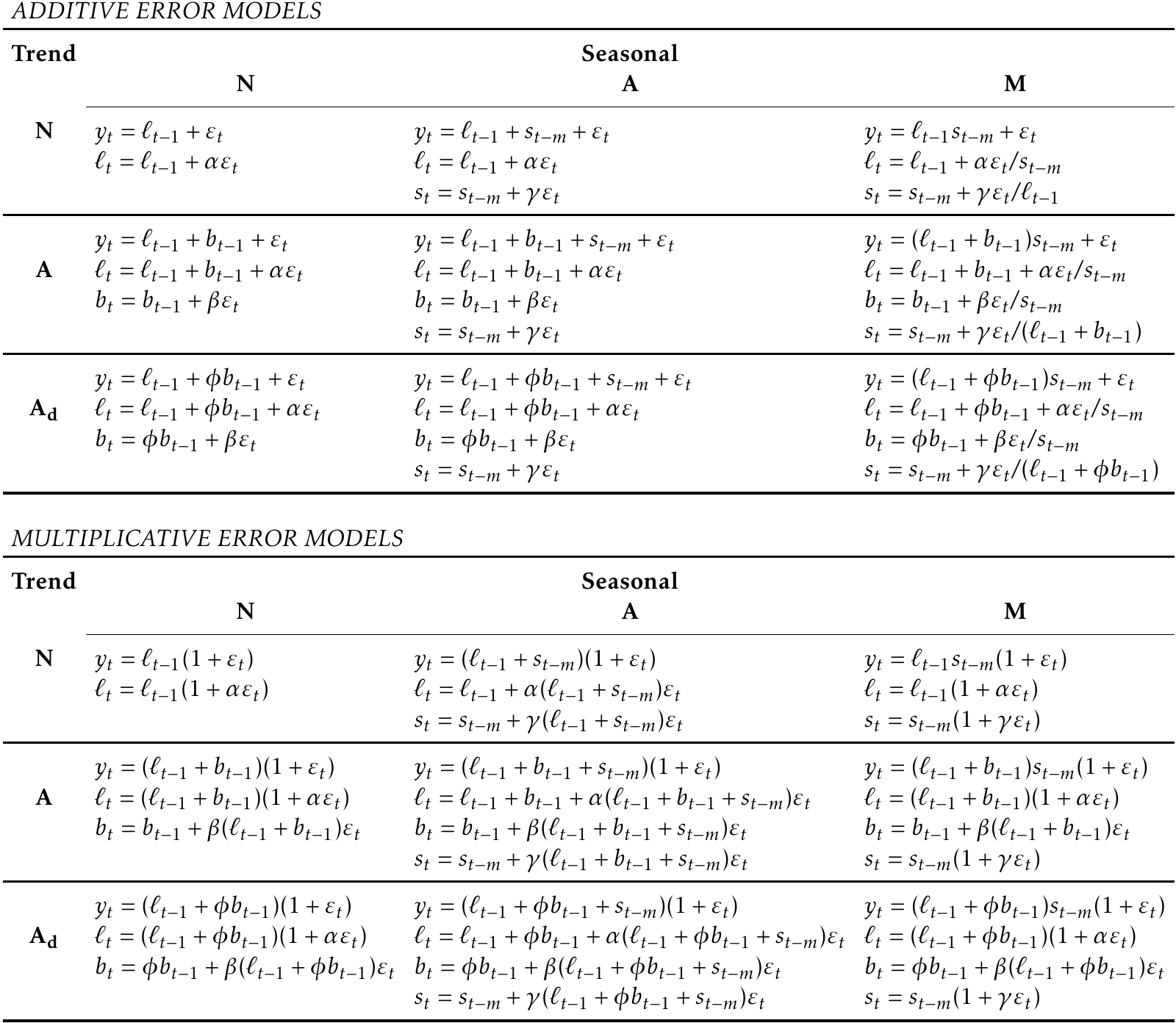
• The concept for state models is that although the prediction algorithms for exponential smoothing provide point forecasts, stochastic models that generate data is what produce the distributions for forecasting.
• Models conain equations for observed data and state equations that describe how the unobserved states(level, trend, season) change over time.
• These models are called innovation state models as they all use the same ε (random error process) for both the forecasting and smoothing equations as seen from the chart for all error models above.

Parameter estimation and selection

• For additive models, minimizing the SSE of the model is the same process to maximizing the 'likelihood".
• Models that minimize AIC(Akaike's Information Criteria) or AICc could be considered as good models as discussed before from regression model evaluations.
• The most important part for model selection is that "Minimizing AIC, assuming ε ~ N(0,σ^2) is equal to a one-step time series cross-validation on MSE"
• Therefore, a good model can be selected on the criteria of a miniziming AIC instead of cross-validating the accuracy of the model.