Random Forest model to forecast energy consumptions
Using the skforecast package, let's try to use a Random Forrest model to predict future energy consumptions in Ontario.
First import the dataset for Ontario's energy consumption, found in IESO's website. The dataset shows hourly data for consumption, so we need to convert it into monthly consumption data.
elec_dat = pd.read_csv('ontario_electricity_demand.csv')

# First, group energy consumption by day
dem_dt = elec_dat.groupby('date').sum()

# Next, group energy consumption by month
dem_dt['month'] = dem_dt['date'].dt.month
dem_dt['year'] = dem_dt['date'].dt.year
dem_dt['year_month'] = pd.to_datetime(dem_dt[['year', 'month']].assign(day=1))
df = pd.DataFrame(dem_dt.groupby('year_month')['daily_dem'].sum())
We now split our dataset between train and test sets. I chose the prediction step 2 years arbitrarily.
steps = 24 # 24months = 2Years
data_train = df[:-steps]
data_test  = df[-steps:]
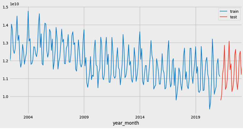
Now, our train/test dataset looks like this.

I want to train both the ARIMA model and the RF model for forecasting the next 2 years.
First, I'll train the ARIMA model. I'm assuming that the ARIMA(2,0,1)(0,1,1) model is the best fit model, which I found it to have the lowest AICc from my project. For further details, check out my project.
import statsmodels
from statsmodels.tsa.statespace.sarimax import SARIMAX

# Train & Fit SARIMA model
model = SARIMAX(endog = data_train, order = (2, 0, 1), seasonal_order = (0, 1, 1, 12))
model_res = model.fit(disp=0)
model_res.summary()

# Make predictions for 2 years
predictions_statsmodels = model_res.get_forecast(steps=len(data_test)).predicted_mean
predictions_statsmodels.name = 'predictions_arima'
Simple as that, we have our predictions for our ARIMA model.
Now, we will use a Random Forest model from sklearn to make our predictions. The hyperparameters for the random forest model include the number of trees to generate (n_estimators), and the depth of each tree(max_depth). For the time series forecasting, we also need the number of lags, which basically determines how many features that we will be using for our random forest.
What I mean by number of features, we are converting a time series into a tabular form of data, which is suitable for regression/classification tasks for a random forest model. The gif below provides a good example of this conversion.

We will iteratively go through a grid search of potential parameters to find the best hyperparameters for our model.
# parameters to be estimated
lags_grid = [3,6,9,12] # lag over 12 months will have correlation!

param_grid = {
    'n_estimators': [100,200,300,500], # n_estimators usually don't overfit a rf tree
    'max_depth': [3,4,5,6] # shallower trees usually perform better
}

grid_search_model = grid_search_forecaster(
                   forecaster         = forecaster,
                   y                  = data_train['y'],
                   param_grid         = param_grid,
                   lags_grid          = lags_grid,
                   steps              = steps,
                   metric             = 'mean_squared_error',
                   initial_train_size = int(len(data_train)*0.5),
                   fixed_train_size   = False,
                   refit              = False,
                   skip_folds         = None,
                   return_best        = True,
                   n_jobs             = 'auto',
                   verbose            = False
               )


# `Forecaster` refitted using the best-found lags and parameters, and the whole data set:
#  Lags: [ 1  2  3  4  5  6  7  8  9 10 11 12]
#  Parameters: {'max_depth': 3, 'n_estimators': 100}
#  Backtesting metric: 4.5836819294469203e+17
Our grid search found that 12 lagged values, max depth of 6, and 300 trees had the lowest MSE. Now we train, fit, and generate our forecasts with this model!
forecaster_rf = ForecasterAutoreg(
                 regressor = RandomForestRegressor(n_estimators=100, max_depth=6, random_state=10),
                 lags      = 12
             )

# fit!
forecaster_rf.fit(y=data_train['y'])
# predict!
predictions = forecaster_rf.predict(steps=24)
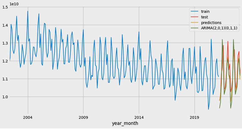
Then plot to see how our models perform against the test set.

Looks like both our models do pretty well here. Let's take a look at its MSE for test error!
error_mse_rf = mean_squared_error(
                y_true = data_test['y'],
                y_pred = predictions
            )
error_mse_arima = mean_squared_error(
                y_true = data_test['y'],
                y_pred = predictions_statsmodels
            )

# Test error (RF): 2.5941181466278016e+17
# Test error (ARIMA): 3.9814703152386195e+17
Seems like the RF did a lot better than the ARIMA. In fact, RF has a 35% lower test MSE! HOWEVER, we should always be very careful not to solely rely on the test MSE.
Cross-validation is always a more accurate measure of accuracy of the model. For this case, we are going to apply backtesting of a rolling origin, with 9 folds, each with 12 steps(1 year) for 10 years.
steps = 12
n_backtesting = 12*10 # 10 years in total or 9 Years because you don't count your first year

# cross-validation for RF
metric_rf, predictions_rf= backtesting_forecaster(
                                   forecaster         = forecaster_rf,
                                   y                  = df['y'],
                                   initial_train_size = len(df) - n_backtesting,
                                   fixed_train_size   = False,
                                   steps              = 12,
                                   metric             = 'mean_squared_error',
                                   refit              = True,
                                   verbose            = True,
                                   show_progress      = True
                               )

# cross-validation for ARIMA
metric_arima, predictions_arima = backtesting_sarimax(
                          forecaster            = forecaster_arima,
                          y                     = df['y'],
                          initial_train_size    = len(df) - n_backtesting,
                          fixed_train_size      = False,
                          steps                 = 12,
                          metric                = 'mean_squared_error',
                          refit                 = True,
                          verbose               = True,
                          show_progress         = True
                      )

metric.rename(index={0:'Random Forrest'}, inplace=True)
metric_arima.rename(index={0:'ARIMA(2,0,1)(0,1,1)'}, inplace=True)

comp_df = pd.concat([metric, metric_arima])

# 	Model                   mean_squared_error
#   -------------------------------------------
#   Random Forest 	        2.766257e+17
#   ARIMA(2,0,1)(0,1,1) 	  2.887092e+17
#
And now, we can see that the random forest model actually has about 5% lower MSE than the ARIMA model compared to the 35% difference from just comparing the test MSE. This is still a good improvement!
Conclusion
Again, I think this shows that ARIMA models are great baseline models that should always be used to test out any other ML models. Cross-validation is also very important to measure the performance of the model as test errors could be misleading.
© Joe Lee.RSS